Report project : Pedestrians Detection with TensorFlow

 

I ) Introduction

 

During the Computer Vision course we had to work on a project. We  chose the Pedestrian Detection subject. The purpose of this task is to detect and locate the pedestrians in the field of view of the camera.

For that, we used an existant algorithm SSD (Single Shot MultiBox Detector). This code is implemented in Python. The Tensorflow library has been used in this one.

In this report, we will explain the VGG16 network. After that, we will introduce the SSD model. Then, we will do some tests in order to see how it works.

 

II ) The VGG16 network

 

The SDD network is based on the VGG16 architecture. So in this section we will explain this architecture.

 

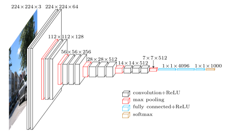
 Figure 1 : VGG16 network

 

This network is called VGG16 because it has 16 layers of neurons.

To build this network we begin by adding two convolutions and we use the Relu activation function after that we do a compression with max pooling. We do the same a second time. Then we add three convolutions and use again the Relu function and the max pooling, we add this part three times.  Then we add three layers of neurons fully connected with the use of the function Relu. And to finish we use softmax like classifier.

Convolution : The convolutional layer is the core building block of a CNN. The layer's parameters consist of a set of learnable filters. Each filter is convolved across the width and height of the input volume, computing the dot product between the entries of the filter and the input and producing an activation map of that filter. As a result, the network learns filters that activate when it detects some specific type of feature at some spatial position in the input.

Adding several convolution allows to a neuron to looks a small region in the input.

Activation function : An activation function of a node defines the output of that node given an input or set of input.

Relu function : The Relu function is defined like this : f(x)=max(0,x).

Pooling layer : The pooling layer serves to progressively reduce the spatial size of the representation, to reduce the number of parameters and amount of computation in the network.

Max pooling : Max pooling is a pooling layer. The most common form is a pooling layer with filters of size 2x2 applied with a stride of 2 downsamples at every depth slice in the input by 2 along both width and height,

 

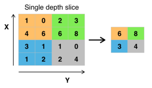Figure 2 : Max pooling with a 2x2 filter and stride = 2

 

 

 

Fully connected layers : After several convolutional and max pooling layers, we need to add fully connected layers. Neurons in a fully connected layer have connections to all activations in the previous layer.

The loss layer  : It specifies how training penalizes the deviation between the predicted and true labels and is normally the final layer.

Softmax loss  : The softmax function is often used in the final layer of a neural network-based classifier. This loss is used for predicting a single class of K mutually exclusive classes.

 

II ) The SSD model

 

SSD is a fast single-shot objet detector for multiple categories. 

The network of the SSD model is the following :

Figure 3 : SDD model

We can see that it is composed by the VGG16 network, it also have several convolutions. At the end there is a non maximum supression algorithm in order to eliminate multiple detections. The detections that have the higher score is selected and all the others are removed from the detection set.

The SSD network that we downloaded is already trained. For restoring it we need do to the following instructions :

ckpt_filename is the file where the trained model is saved.

If we want to use it we have to give an image to network.

The function process_image give this image to the network and returns the classes, the scores and positions of the boxes.

The function visualization.plt_bboxes returns the initial image with the boxes plotted and the number of the class and its percentage.

We have seen it the code that the total number of classes is 21.

 

III ) Network tests

 

In this part we wil examine the performance of this network by giving it different images.

First we will give it an image from the database Demo.

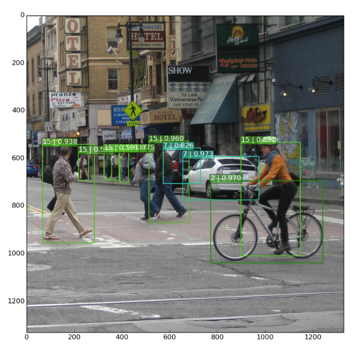
Figure 4 : Example of objets detection in a image

 

The figure 3 show the image that the algorithm returns. We can see that is able to recognize pedestrians and also others objets like cars and bike. In the image we have a colored box around each objet detected. For each class we have a box in a specific color with the number that represents this class. In these boxes we also have the percentage of chance that the objet is well detected.

We can notice that the pedestrians have the number fifteen. We remark that the pedestrians in the foreground of the image are better detected than the others in the background.

With this example we can say that pedestrians are well detected.

Now we will take another image that doesn't come from the database demo to compare.

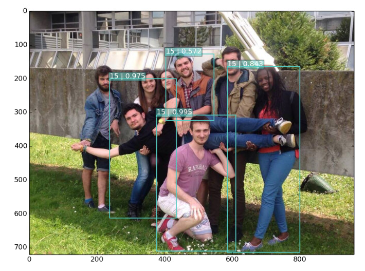
Figure 5 :  Example of pedestrians detection in an image.

 

In this picture there are eight people and the algorithm detects only four of them.

For the box with the percentage 0.975 we don't know which person is detected. It could be the girl or the man in the horizontale.

Therefore even if we have high percentage it doesn't mean that the algorithm has well detected the object.

 

IV) Conclusion

 

To conclude, we  presented the VGG 16 network . Then, we introduced the SSD network which use the VGG architecture. After that, we did some tests to evaluate the efficiency of this model. Thanks to these tests we noticed that pedestrians are not always well detected even if the percentage is high.

The next part of this project will be to modify the code in order to make it able to identify only pedestrians.